12 Ramp Metering
12.1 Introduction
Ramp metering is used to control the flow of freeway on-ramp vehicles onto the mainline in an effort to prevent freeway flow breakdown, as well as improve the safety of merging operations. Determining effective ramp metering rates can be a complicated process because of the need to usually balance freeway, ramp, and arterial flows. Numerous ramp-metering algorithms have been developed. SwashSim currently implements the following algorithms:
- Pretimed
- Demand/Capacity
- ALINEA
- Fuzzy logic
12.2 Pretimed
With pretimed ramp metering, the ramp signal operates with a constant cycle in accordance with a metering rate prescribed for a particular control period. With this approach, the fixed ramp rates are usually based on historical traffic observations, assuming that traffic patterns are fairly consistent. Advantages of the pretimed algorithm is that it is relatively low cost because detection infrastructure is not needed, and it also can effectively relieve localized recurrent congestion. The major disadvantage is that the system can neither respond automatically to significant changes in demand, nor adjust to unusual traffic conditions resulting from incidents.
12.3 Demand/Capacity
With demand/capacity control, the on-ramp flow is determined as the difference between the upstream freeway flow (or occupancy) and the downstream capacity (or desired occupancy). The measurement of the freeway flow or occupancy occurs in real-time (i.e., measured in the previous time interval). The on-ramp flow is then expressed as the metering rate for the next control interval, based on the equation:
\[R(t) = c - q(t-1)\]
where:
\({R(t)}=\) ramp−metering rate at time interval t,
\(c=\) capacity of freeway section (predefined), and
\(q(t-1)=\) upstream flow rate at time (t-1) (measured).
This algorithm requires detectors to be located on the freeway mainline, immediately upstream of the merge point and downstream of the merge point. This method of control offers improvements over the pretimed method in that it can respond automatically to changes in traffic flow; however, detection is required. Disadvantages to this method include 1) measurement of the upstream freeway flow rate alone is not sufficient to determine whether the freeway is congested or free-flowing; and 2) for optimal system operation, accurate estimates of capacity are required. Alternatively, the algorithm can be based on occupancy measures instead of flow measures. The occupancy strategy relies on occupancy-based estimation of the upstream freeway flow. If the aggregated occupancy on the freeway downstream detector is above the critical occupancy, it hits the minimum metering rate, otherwise the metering rate is set as the difference between the capacity at the downstream detector and aggregated flow rate at the upstream detector. The demand/capacity algorithm logic is illustrated in the following figure.
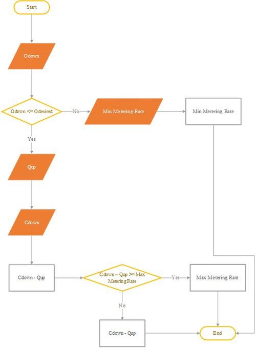
Figure 12.1: Demand/Capacity Algorithm Logic
where:
\(O_{down}=\) aggregated freeway occupancy downstream of merge point,
\(O_{desired}=\) desired aggregated freeway occupancy downstream of merge point (considered as 20%),
\(Q_{up}=\) aggregated freeway flow rate immediately upstream of merge point (veh/h),
\(C_{down}=\) freeway capacity downstream of merge point (veh/h),
MinMeteringRate = typically 180-240 veh/h, and
MaxMeteringRate = typically 900-1200 veh/h.
12.4 ALINEA
ALINEA is a simple but effective ramp metering strategy that utilizes a local traffic-responsive feedback loop to maintain maximum throughput at the downstream merge area of an on-ramp. The ALINEA algorithm calculates the metering rate at each time step by computing the difference between the downstream desired occupancy and the aggregated downstream occupancy at each time step, multiplying that difference by a regulator parameter, and adding that result to the metering rate of the previous time step. The following equation implicitly calculates the metering rate:
\[r(k) = r(k-1) + {K_{R}}\times \big(\hat{O}-{O_{Out}}(k)\big)\]
where:
\({r(k)}=\) ramp−metering rate at time index k,
\({K_{R}}=\) constant regulator,
\(\hat{O}=\) desired downstream occupancy,
\({O_{Out}}(k)=\) aggregated downstream occupancy at time index k.
Detectors are placed on every freeway lane 500 m downstream of the acceleration lane. The detector data for each lane is aggregated together at each time step to calculate the occupancy value that is compared to the desired occupancy. The on-ramp contains two detectors: a presence detector directly behind the ramp meter signal controller and a passage detector immediately after the ramp meter signal controller. The presence detector ensures that the signal rests on red when no vehicles are detected and ensures that the ramp metering algorithm is being applied when a vehicle is detected. The passage detector ensures that the system does not break down in case vehicles stay queued up behind the signal controller. The figure below illustrates the ALINEA setup used in SwashSim.
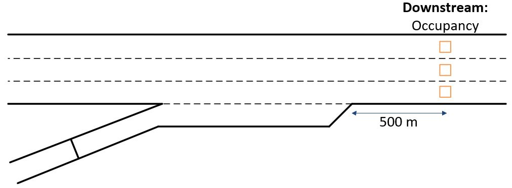
Figure 12.2: Detector Setup for ALINEA Algorithm
The ALINEA flow chart below reads as follows:
- Start.
- Set time step to 1.
- Calculate the downstream mainline occupancy at the current time step.
- Calculate the metering rate using the occupancy calculated in Step 3.
- Check if the calculated metering rate is less than the minimum metering rate. If yes, set the calculated metering rate to the minimum metering rate.
- If the calculated metering rate is higher than the minimum metering rate, check if the calculated metering rate is greater than the maximum metering rate. If yes, set the calculated metering rate to the maximum metering rate.
- Advance to the time step and repeat.
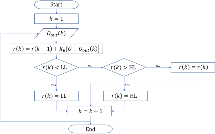
Figure 12.3: ALINEA Algorithm Logic
where:
\(LL=\) low limit (minimum) metering rate, and
\(HL=\) high limit (maximum) metering rate.
For more information, see Papageorgiou, Hadj-Salem, and Blosseville (1991).
12.5 Fuzzy Logic
Another method through which ramp metering can be integrated into SwashSim is fuzzy logic. Fuzzy-logic algorithm was developed in response to the limitations of the Seattle bottleneck algorithm (i.e., it addresses the inherent issues with data accuracy and reliability in loop detectors, optimizes the mainline congestion and the ramp queues, does not require extensive system modeling, and is easy to tune using linguistic variables rather than numerical variables). This algorithm uses the mainline speed and occupancy and the ramp occupancy to calculate metering rates. This algorithm has nine rule groups including the upstream speed, upstream occupancy, upstream flow, downstream speed, downstream v/c, ramp demand occupancy, ramp queue occupancy the ramp occupancy, and ramp metering. Each rule group is associated with one or more of the six fuzzy classes including very low (VL), low (L), medium (M), high (H), and very high (VH). Ramp meters are calculated based on the rule weight and the degree of activation of each rule outcome. The location of each of the detectors are the same as the ones shown in ALINEA; however, there are additional detectors located upstream immediately at the end of the ramp. The figure below illustrates the Fuzzy Logic setup used in SwashSim.
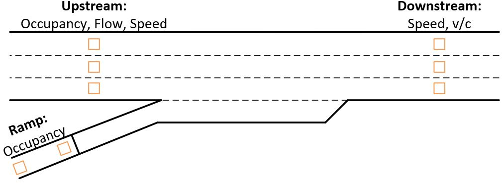
Figure 12.4: Detector Setup for Fuzzy Logic Algorithm
The graphic below is an example of a typical fuzzy logic system. The following is a description of the major components of the fuzzy logic system:
- Fuzzifier: The fuzzifier translates each input into a set of fuzzy variables via membership functions.
- Rules: The rules are the set of regulations that are based on expert opinions.
- Inference: The inference stage involves applying fuzzy operators and implication methods to the rule base, allowing the fuzzy inputs to be converted into one fuzzy output.
- Defuzzifier: The defuzzifier produces a crisp output based upon the fuzzy output.
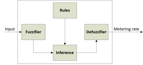
Figure 12.5: Fuzzy Logic Algorithm Logic
Fuzzy Sets
The fuzzification process involves translating each input into a fuzzy set with understandable terms such as “low” and “high”. This is done using membership functions, which are different for each input type. Upstream mainline inputs use the Gaussian function, downstream mainline and ramp inputs use the Sigmoid function, and the output uses the triangular function. The full list of inputs along with their specific fuzzy sets and membership functions is shown below.
| Input | Fuzzy Set | Membership Function |
|---|---|---|
| Upstream mainline | ||
| Occupancy | Low Medium High | Gaussian |
| Flow | Low Medium High | Gaussian |
| Speed | Low Medium High | Gaussian |
| Downstream mainline | ||
| Speed | Very low | Sigmoid |
| v/c | Very high | Sigmoid |
| Ramp | ||
| Demand Occupancy | Very high | Sigmoid |
| Queue Occupancy | Very high | Sigmoid |
| Output | ||
| Metering rate | Low Medium High | Triangular |
12.5.1 Inputs (Aggregated Performance Measures)
Aggregated Upstream Mainline Occupancy
Considering the aggregated upstream mainline occupancy varies from 0 to 20% and is described as 3 Gaussian fuzzy sets: Low, medium, and high. The overlap is 50% and the parameters (center point and the sigma value) are found below.
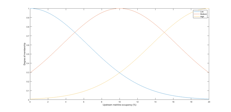
Figure 12.6: Fuzzy Logic Upstream Occupancy
\[Guassian(x;c,σ) = e^{-\frac{1}{2}(\frac{x-c}{σ})^{2}}\]
| Fuzzy Set | c (%) | \(\sigma\) (%) |
|---|---|---|
| Low | 0 | 6.4 |
| Medium | 10 | 6.4 |
| High | 20 | 6.4 |
Aggregated Upstream Mainline Flow
Considering the upstream mainline flow varies from 0 to 2,000 veh/h/ln and is described as 3 Gaussian fuzzy sets: Low, medium, and high. The overlap is 50% and the parameters (center point and the sigma value) are found below.
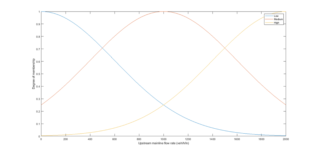
Figure 12.7: Fuzzy Logic Upstream Flow
\[Guassian(x;c,σ) = e^{-\frac{1}{2}(\frac{x-c}{σ})^{2}}\]
| Fuzzy Set | c (veh/h/ln) | \(\sigma\) (veh/h/ln) |
|---|---|---|
| Low | 0 | 601 |
| Medium | 1000 | 601 |
| High | 2000 | 601 |
Aggregated Upstream Mainline Average Speed
Considering the aggregated upstream mainline average speed varies from 0 to 100 km/h and is described as 3 Gaussian fuzzy sets: Low, medium, and high. The overlap is 50% and the parameters (center point and the sigma value) are found using the plot shown below.
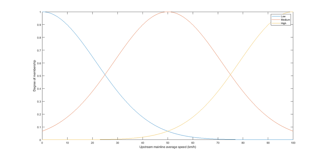
Figure 12.8: Fuzzy Logic Upstream Flow
\[Guassian(x;c,σ) = e^{-\frac{1}{2}(\frac{x-c}{σ})^{2}}\]
| Fuzzy Set | c (km/h) | \(\sigma\) (km/h) |
|---|---|---|
| Low | 0 | 21.5 |
| Medium | 50 | 21.5 |
| High | 100 | 21.5 |
Aggregated Downstream Mainline Average Speed
Aggregated downstream mainline average speed varies from 0 to 110 km/h. It is described as only 1 Sigmoid fuzzy set which is very low, and the parameters (center point and the sigma value) are found using the plot shown below.
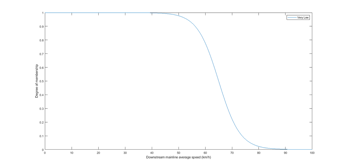
Figure 12.9: Fuzzy Logic Upstream Flow
\[Sig(x;a,c) = \frac{1}{1+e^{-a(x-c)}}\]
| Fuzzy Set | c (km/h) | a (km/h) |
|---|---|---|
| Very Low | 65 | \(-0.25\) |
Aggregated Downstream Mainline v/c
Aggregated Downstream mainline v/c ratio varies from 0 to 1. It is described as only 1 Sigmoid fuzzy set which is very high, and the parameters (center point and the sigma value) are found using the plot shown below.
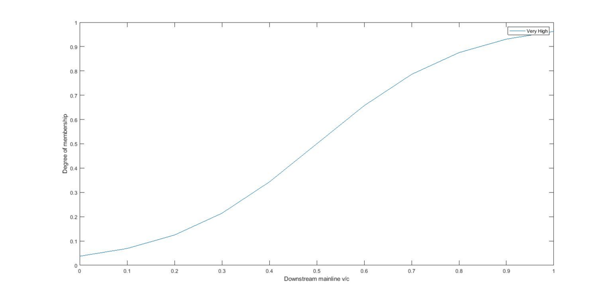
Figure 12.10: Fuzzy Logic Upstream Flow
\[Sig(x;a,c) = \frac{1}{1+e^{-a(x-c)}}\]
| Fuzzy Set | c (unitless) | a (unitless) |
|---|---|---|
| Very High | 0.5 | 6.5 |
Aggregated Ramp Demand/Queue Occupancy
Both the aggregated ramp demand and queue occupancy vary from 0 to 50% described as only 1 Sigmoid fuzzy set which is very high, and the parameters (center point and the sigma value) are found using the plot shown below.
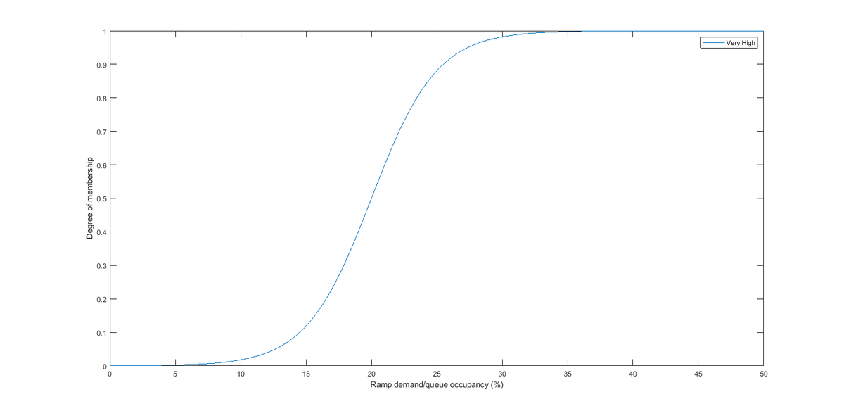
Figure 12.11: Fuzzy Logic Upstream Flow
\[Sig(x;a,c) = \frac{1}{1+e^{-a(x-c)}}\]
| Fuzzy Set | c (%) | a (%) |
|---|---|---|
| Very High | 20 | 4 |
12.5.2 Inference
Fuzzy logic relationship will be defined as a list of if-then pairs between the inputs condition and the outputs responses. The inputs condition is a “premise” and the out responses is a “consequent” (Yu (2009)). For example, as shown in the diagram below, the Rule Condition starts with a If and the Rule Outcome starts with a then. Within the rule condition, there is a AND or OR operation. The AND operation is analogous to the intersection of fuzzy sets, which takes the minimum value of given degree of membership which is between 0-1. The OR operation is analogous to the union of fuzzy sets, which takes the maximum value of given degree of membership which is between 0-1.
| Rule # | Rule Weight | Inference | Outcome |
|---|---|---|---|
| 1 | 1.5 | If upstream mainline occupancy is low | Metering rate is high |
| 2 | 1.5 | If upstream mainline occupancy is medium | Metering rate is medium |
| 3 | 2.0 | If upstream mainline occupancy is high | Metering rate is low |
| 4 | 2.0 | If upstream mainline flow is high AND upstream mainline speed is low | Metering rate is low |
| 5 | 1.0 | If upstream mainline occupancy is high AND upstream mainline speed is medium | Metering rate is medium |
| 6 | 1.0 | If upstream mainline occupancy is low AND upstream mainline speed is medium | Metering rate is high |
| 7 | 1.0 | If upstream mainline flow is low AND upstream mainline speed is high | Metering rate is high |
| 8 | 3.0 | If downstream mainline speed is very low AND downstream mainline v/c is very high | Metering rate is low |
| 9 | 3.0 | If ramp demand occupancy is very high OR ramp queue occupancy is very high | Metering rate is high |
Rules 1 to Rule 3 The purpose of rule 1 through rule 3 is to form a complete rule base, which means at least one of the rules would work since the whole occupancy range is covered.
Rule 4 to Rule 7 The purpose of rule 4 to 7 is to couple speeds with either occupancy or flow to generate metering rates according to the fundamental diagram of traffic flow
Rule 8 The purpose of rule 8 is to prevent the formation of downstream congestion. v/c-ratio calculated with the historical measured maximum flow rate of downstream can be seen as a prediction of the downstream bottleneck behavior.
Rule 9 The purpose of rule 9 is to prevent the excessive queue formation and to avoid a spillback onto the arterial street road by applying the information collected from queue detector.
Rule weights The rule weight is to stress the priority of each rule. Rule weighting scheme is flexible for different applications.
12.5.3 Output (Ramp Metering)
The metering rate varies from 240 veh/h to 900 veh/h, and is described as 3 triangular fuzzy sets: Low, medium, and high. The overlap is 50%.
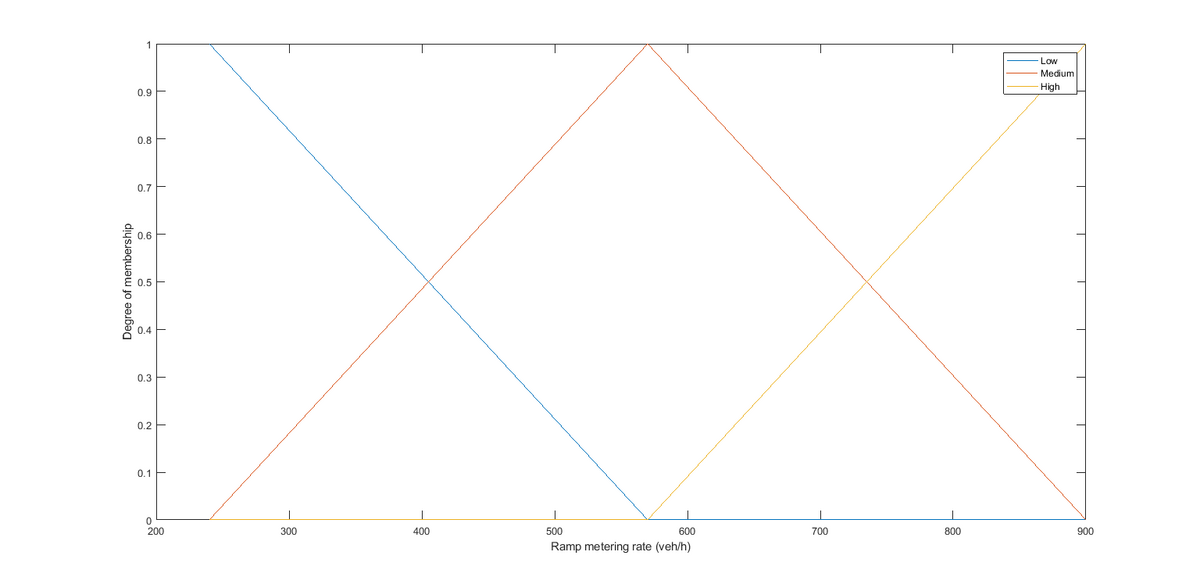
Figure 12.12: Fuzzy Logic Upstream Flow
| Fuzzy Set | a (veh/h) | b (veh/h) | c (veh/h) |
|---|---|---|---|
| Low | 240 | 240 | 570 |
| Medium | 240 | 570 | 900 |
| High | 570 | 900 | 900 |
\[ Triangle(x;a,b,c)=\left\{\begin{array}{l} 0,& \mbox{x $\leq$ a}\\ \frac{x-a}{b-a},& \mbox{a $\leq$ x $\leq$ b}\\ \frac{c-x}{c-b},& \mbox{b $\leq$ x $\leq$ c}\\ 0,& \mbox{x $\geq$ c} \end{array}\right. \]
Defuzzification
The defuzzication process is to convert a fuzzy output variable into a crisp value (metering rate). The centroid method is commonly used for the defuzzification process. In practice, a discrete fuzzy centroid equation is used to replace the continuous centroid equation since it is easier to calculate. The equation is shown below.
\[Metering Rate = \frac{\sum^3_{i=1}{w_{i}}{c_{i}}{I_{i}}}{\sum^3_{i=1}{w_{i}}{c_{i}}}\]
where:
\({w_{i}}=\) weighted output for fuzzy set i,
\({c_{i}}=\) centroid of fuzzy set i, and
\({I_{i}}=\) area of fuzzy set i.
The indices from the rule outcome refers to the rule # mentioned under inference.
\(w(Low) = RuleOutcome[3] \times 2 + RuleOutcome[4] \times 2 + RuleOutcome[8] \times 3\),
\(w(Medium) = RuleOutcome[2] \times 1.5 + RuleOutcome[5] \times 1\),
\(w(High) = RuleOutcome[1] \times 21.5 + RuleOutcome[6] \times 1 + RuleOutcome[7] \times 1 + RuleOutcome[9] \times 3\), and
\(c(Low) = \frac{c-b}{3} + a\)
\(c(Medium) = b\),
\(c(High) = c - \frac{b-a}{3}\),
\(I(Low) = 165\),
\(I(Medium) = 330\), and
\(I(High) = 165\).