25 Car Following
If a vehicle is considered to be a follower, the program will calculate an acceleration value for this vehicle according to a car-following model. This calculated acceleration is also subject to the following constraints:
- the vehicle’s maximum acceleration
- the vehicle’s maximum deceleration
- safe following distance; that is, if the lead vehicle decelerates at its maximum value, the acceleration of the following vehicle must not move it so close to the lead vehicle such that it would not be able to stop before colliding with the lead vehicle in this situation.
If the vehicle is not considered to be a follower, the calculation of an acceleration according to a car-following model is skipped. The determination of whether or not a vehicle is in a follower status is described here.
SwashSim employs the Modified-Pitt car-following model (Cohen (2002a) and Cohen (2002b)). The Modified-Pitt car-following model has been demonstrated (Cohen (2002a) and Cohen (2002b); Washburn and Cruz-Casas (2010)) to work well for multiple traffic flow regimes (e.g., uninterrupted flow and queue arrival/discharge flow).
The Modified-Pitt car-following equation calculates the acceleration value for a trailing vehicle based on intuitive parameters such as the speed and acceleration of the lead vehicle, the speed of the trailing vehicle, the relative position of the lead and trail vehicles, as well as a desired headway. This equation also incorporates a sensitivity factor, K, which is discussed in the next subsection. This equation allows for relatively easy calibration. Car-following models are generally based on a ‘driving rule’, such as a desired following distance or following headway. The Modified-Pitt model is based on the rule of a desired following headway. The main form of the model is as follows.
\[{a_f}(t+T)=K\frac{{s_l}(t+R)-{s_f}(t+R)-{L_l}-h{v_f}(t+R)+[{v_f}(t+R)-{v_l}(t+R)]T-\frac{1}{2}{a_l}(t+T)T^2}{T(h+\frac{1}{2T})}\]
where:
\({a_f}(t+T) = \text{acceleration of follower vehicle at time } t+T \text{ (ft/s}^2)\),
\({a_l}(t+T) =\) acceleration of lead vehicle at time \(t+T \text{ (ft/s}^2)\),
\({s_l}(t+R) =\) position of lead vehicle at time \(t+R\) as measured from upstream (ft),
\({v_f}(t+R) =\) speed of follower vehicle at time \(t+R\) (ft/s),
\({v_l}(t+R) =\) speed of lead vehicle at time \(t+R\) (ft/s),
\({L_l} =\) length of lead vehicle plus a buffer based on jam density (ft),
\({h} =\) time headway parameter (refers to headway between rear bumper plus a buffer of lead vehicle to front bumper of follower) (s),
\({T} =\) simulation time-scan interval (s),
\({t} =\) current simulation time step (s),
\({R} =\) perception-reaction time (s), and
\({K} =\) sensitivity parameter (unitless).
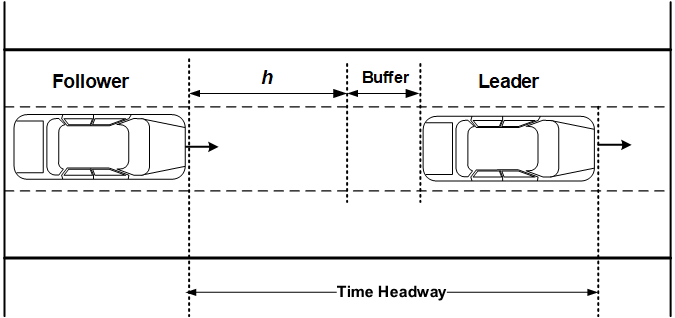
Figure 25.1: Car-following Illustration
The ‘’K’’ value is a sensitivity parameter used to adjust the acceleration calculated by the car-following model. This factor is analogous to a spring constant used to describe how tightly or loosely a coupled system (a platoon of vehicles in this case) operates. This factor essentially adjusts how quickly or slowly acceleration changes, for one or more vehicles, propagate through the platoon.
By default, two separate values for the sensitivity parameter, K, are used in the car-following model—one for uninterrupted flow and one for queue arrival/discharge flow. Cohen stated that a larger K value should be used in interrupted flow conditions (a more tightly coupled system) due to over-damping effects (Cohen (2002b)). This assumption was tested in a work zone simulation situation (Washburn, Watson, and Song (2014)) and was found to yield good results. Vehicles had a smoother interaction in the work zone (uninterrupted flow, a more loosely coupled system) with K = 0.75 and the queue arrival and queue discharge processes performed well with K = 1.1. The definition of the queue arrival area was 300 ft upstream of the last vehicle in the queue, and the definition of the queue discharge area was 300 ft downstream of a stop bar (see Figure below). These values can be revised in the Settings, under the ‘Car Following’ section.
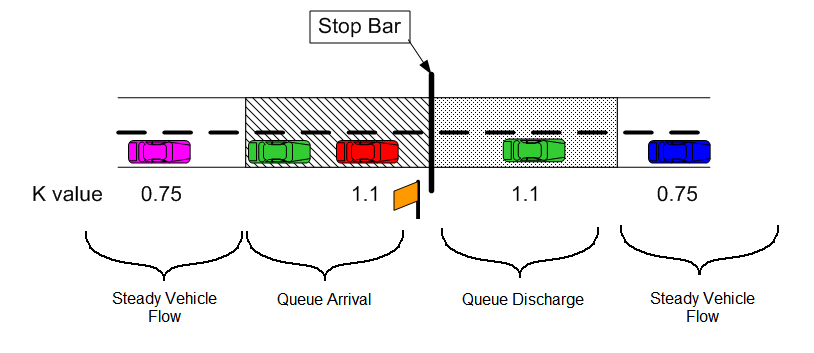
Figure 25.2: Modified-Pitt K-values