26 Maximum Acceleration
The approach used to model vehicle maximum acceleration in SwashSim is based on the vehicle performance theory and equations given in Principles of Highway Engineering and Traffic Analysis (Mannering and Washburn (2019)). This approach utilizes detailed information about a vehicle’s physical and powertrain characteristics. An overview of this approach is given here.
The approach at its most basic level determines acceleration through the fundamental equation relating tractive force to resistance forces, as follows.
\[F=ma+{R_a}+{R_{rl}}+{R_g}\]
The tractive force, F, referred to here as available tractive effort, is taken as the lesser of maximum tractive effort and engine-generated tractive effort. Maximum tractive effort is a function of several of the vehicle’s physical characteristics (such as wheelbase, center of gravity, and weight) and the roadway coefficient of road adhesion. Maximum tractive effort represents the amount of longitudinal force that can be accommodated by the tire-pavement interface. Engine-generated tractive effort is a function of engine torque, transmission and differential gearing, and drive wheel radius. For vehicles with low power-to-weight ratios, such as commercial trucks, maximum tractive effort is very rarely the governing condition. Thus, the acceleration calculations for trucks in SwashSim are based on engine-generated tractive effort.
The major resistance forces are aerodynamic, rolling, and grade. The equation for determining aerodynamic resistance is
\[{R_a}=\frac{\rho}{2}{C_D}{A_f}{V^2}\]
where:
\({R_a}=\) aerodynamic resistance (lb),
\(\rho=\) air density (slugs/ft\(^3\)),
\({C_D}=\) coefficient of drag (unitless),
\({A_f}=\) frontal area of the vehicle (projected area of the vehicle in the direction of travel) (ft\(^2\)), and
\({V}=\) vehicle speed (ft/s).
The coefficient of rolling resistance for road vehicles operating on paved surfaces is approximated as
\[{f_{rl}}=0.01(1+\frac{V}{147})\]
where:
\({f_{rl}}=\) coefficient of rolling resistance (unitless), and
\({V}=\) vehicle speed (ft/s).
The rolling resistance, in lb, is simply the coefficient of rolling resistance multiplied by \({W \cos \theta_g}\), the vehicle weight acting normal to the roadway surface. For most highway applications \({\theta_g}\) is very small, so it can be assumed that \({\cos \theta_g} = 1\), giving the equation for rolling resistance (\({R_{rl}})\) as
\[{R_{rl}}={f_{rl}}W\]
Grade resistance is simply the gravitational force (the component parallel to the roadway) acting on the vehicle. The expression for grade resistance (\({R_g})\) is
\[{R_g}=W\sin{\theta_g}\]
As in the development of the rolling resistance formula, highway grades are usually very small, so \({\sin \theta_g \tan \approx \theta_g}\). Thus, grade resistance is calculated as
\[{R_g}\approx W\tan{\theta_g}=WG\]
where:
\({G}=\) grade, defined as the vertical rise per some specified horizontal distance (ft/ft).
Grades are generally specified as percentages for ease of understanding. Thus a roadway that rises 5 ft vertically per 100 ft horizontally (\({G} = 0.05\) and \({\theta_g} = 2.86^\circ\)) is said to have a 5% grade.
The relationship between vehicle speed and engine speed is
\[V=\frac{2\pi r{n_e}(1-i)}{\varepsilon_0}\]
where:
\({V}=\) vehicle speed (ft/s),
\({n_e}=\) engine speed (crankshaft revolutions/s),
\({i}=\) slippage of the drive axle, and
\({\epsilon_0}=\) overall gear reduction ratio.
The overall gear reduction ratio is a function of the differential gear ratio and the transmission gear ratio, which is a function of the selected transmission gear for the running speed. This equation can be rearranged to solve for engine speed given the current vehicle speed (if vehicle speed is zero, engine speed is a function of throttle input).
With the calculated engine speed, the torque being produced by the engine can be determined from the torque-engine speed relationship. For example, assuming an engine speed of 2000 revolutions/min with the torque-engine speed relationship (Paccar PX-7 Engine) shown in the following figure, the resulting torque is 660 ft-lb.
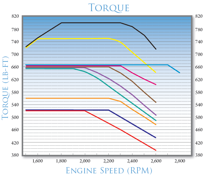
Figure 26.1: Torque-Engine Speed Curve for a Paccar PX-7 Engine (Washburn and Ozkul (2013))
In addition, the figure below illustrates the torque-engine speed relationship for a Paccar MX-13 engine.
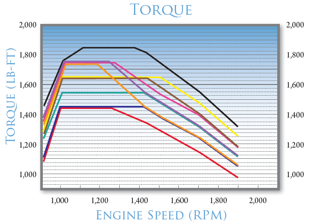
Figure 26.2: Torque-Engine Speed Curve for a Paccar MX-13 Engine (Washburn and Ozkul (2013))
Power is the rate of engine work, expressed in horsepower (hp), and is related to the engine’s torque by the following equation:
\[h{p_e}=\frac{2\pi {M_e}{n_e}}{550}\]
where:
\({hp_\epsilon}=\) engine-generated horsepower (1 horsepower equals 550 ft-lb/s),
\({M_\epsilon}=\) engine torque (ft-lb), and
\({n_\epsilon}=\) engine speed (crankshaft revolutions/s).
The engine-generated tractive effort reaching the drive wheels is given as:
\[{F_e}=\frac{{M_e}{\varepsilon_0}{\eta_d}}{r}\]
where:
\({F_\epsilon}=\) engine-generated tractive effort reaching the drive wheels (lb),
\({M_\epsilon}=\) engine torque (ft-lb),
\({\epsilon_0}=\) overall gear reduction ratio,
\({\eta_d}=\) mechanical efficiency of the drivetrain, and
\({r}=\) radius of the drive wheels (ft).
Note that since torque and horsepower are directly related, if only a power-engine speed relationship is available, this can be converted to a torque-engine speed relationship through the above equation.
For determining vehicle acceleration, the following equation is rearranged and an additional term, \({\gamma_m}\), to account for the inertia of the vehicle’s rotating parts that must be overcome during acceleration, is included.
\[a=\frac{F-\sum R}{{\gamma_m}m}\]
\({\gamma_m}\), referred to as the mass factor, is approximated as:
\[{\gamma _m}=1.04+0.0025\varepsilon_0^2\]
| Vehicle Characteristics | Passenger Car | Single Unit Truck | Intermediate Semi-Trailer | Interstate Semi-Trailer | Semi-tractor+double-trailer |
|---|---|---|---|---|---|
| Vehicle Height (ft) | 4.46 | 10.00 | 10.00 | 10.00 | 10.00 |
| Vehicle Width (ft) | 5.74 | 7.00 | 8.00 | 8.00 | 8.00 |
| Vehicle Length (ft) | 16.00 | 29.00 | 55.00 | 68.50 | 74.60 |
| Vehicle Weight (lb) | 3060 | 25000 | 37000 | 53000 | 55000 |
| Maximum Torque (lb-ft) | 139 | 660 | 1650 | 1650 | 1650 |
| Maximum Power (hp) | 197 | 300 | 485 | 485 | 485 |
| Wheel Radius (ft) | 1.03 | 1.66 | 1.66 | 1.66 | 1.66 |
| Differential Gear Ratio | 4.77 | 4.40 | 3.50 | 3.50 | 3.50 |
| Transmission Gear Ratio | Passenger Car | Single Unit Truck | Intermediate Semi-Trailer | Interstate Semi-Trailer | Semi-tractor+double-trailer |
|---|---|---|---|---|---|
| Gear 1 | 3.27 | 7.59 | 11.06 | 11.06 | 11.06 |
| Gear 2 | 2.13 | 5.06 | 8.20 | 8.20 | 8.20 |
| Gear 3 | 1.52 | 3.38 | 6.06 | 6.06 | 6.06 |
| Gear 4 | 1.15 | 2.25 | 4.49 | 4.49 | 4.49 |
| Gear 5 | 0.92 | 1.50 | 3.32 | 3.32 | 3.32 |
| Gear 6 | 0.66 | 1.0 | 2.46 | 2.46 | 2.46 |
| Gear 7 | N/A | 0.75 | 1.82 | 1.82 | 1.82 |
| Gear 8 | N/A | N/A | 1.35 | 1.35 | 1.35 |
| Gear 9 | N/A | N/A | 1.00 | 1.00 | 1.00 |
| Gear 10 | N/A | N/A | 0.74 | 0.74 | 0.74 |
Additional information about how this methodology is incorporated into simulation is described in Washburn and Ozkul (2013) and Ozkul (2014).