Chapter 10 Introduction to Traffic Simulation

10.1 What is Simulation?

Dictionary definition: The representation of the behavior or characteristics of one system through the use of another system, esp. a computer program designed for the purpose.

A definition more specific to our purposes: A numerical technique for conducting experiments on a computer, which may include stochastic characteristics, be microscopic or macroscopic in nature, and involve mathematical models that describe the behavior of a system over extended periods of real time.

Simulation tools, or programs, utilize a collection of mathematical models and algorithms in representing the transportation system.

10.2 Terminology

The term ‘model’ gets applied almost universally to any concept involving simulation (i.e., ‘simulation model’), but it is important to understand that there are several different contexts in which this may apply.

First, more generally, a model could be one of the following (not an exhaustive list):

• Physical
• Analytical
• Simulation

Physical models are usually applied in situations where the real system can be significantly reduced in scale. Thus, they have very limited application in transportation engineering, primarily because of the difficulty of downsizing humans.

Analytical models may be a single equation that relates one or more independent variables to a dependent variable. Many of the HCM equations fall into this category, for example:

Total lane-changing rate for weaving vehicles:
\[{LC}_{W}={LC}_{MIN} + 0.39\lbrack\left(L_{S} - 300 \right)^{0.5} \times N^2 \times {(1 + ID)}^{0.8}\rbrack\]

Proportion of vehicles remaining in lanes 1 and 2 of on-ramp merge area: \[{P}_{FM} = 0.2178 - 0.000125{v}_{R} + 0.01115 \bigg(\frac{{L}_{A}}{{S}_{FR}}\bigg)\]

It can be defined more broadly as well, as is done in the HCM, as follows: A procedure that uses one or more algorithms to produce a set of numerical outputs describing the operation of a highway segment or system, given a set of numerical inputs.

Another useful term is ‘algorithm’. Dictionary definitions of algorithm include:

• a procedure for solving a mathematical problem in a finite number of steps that frequently involves repetition of an operation
• a step-by-step procedure for solving a problem or accomplishing some end

The HCM defines algorithm as: A set of rules for solving a problem in a finite number of steps.

An algorithm often includes one or more analytical models.

Simulation, again, generally refers to a computerized representation of a real-life system. Within a traffic simulation, multiple algorithms are usually employed to model the various features of the transportation system (roadway, vehicles, control devices, etc.). Thus, when the term ‘simulation model’ is used, it should be understood to mean the application of simulation to model the various aspects of a transportation system. ‘Simulation model’ should not be used as a synonym for a traffic simulation software program or tool. Specific traffic simulation software programs (e.g., SwashSim, CORSIM, VISSIM, Aimsun, TransModeler, etc.) are just that, ‘software programs’ or ‘software tools’, not ‘models’.

Said another way, a simulation software tool (e.g., VISSIM) utilizes a collection of analytical models and algorithms to provide one with the ability to create a virtual model of a transportation system.

10.3 Why use simulation?

• Scenario is too complicated to solve by analytical methods
  
• Scenario is too expensive to test in the field
  
• Scenario is too dangerous to test in the field
  
• Can easily test varying traffic scenarios
  
• Can test identical traffic scenarios on various model alternatives
  
• Can experiment with new situations that do not currently exist
  
• System can be studied in real time or compressed time

10.4 Simulation Modeling Approaches

10.4.1 Spatial and Temporal Level of Detail

• Microscopic: Individual vehicle/person movements are modeled and tracked
  
• Macroscopic: Performance measures are based on aggregate relationships (e.g., flow-speed-density)
  
• Mesoscopic: Individual vehicles are tracked, but simpler models for car-following, lane-changing, etc. are used. Also may be event-based rather than time-step based, or time-step resolution may be decreased.
  
• Hybrid: combination of different approaches

10.4.2 Stochastic

• Input values and model parameters are varied randomly
  • Most applicable to microscopic simulations
    
• Based on probabilistic distributions
  • e.g., Poisson (or Neg. Exp.) for vehicle arrivals
    
• For specific inputs (using distribution parameters, such as mean and std. dev.), outputs will vary

10.4.3 Deterministic

• Input values and model parameters are explicitly known for explicit times
  • e.g., vehicle headways are generated according to a uniform distribution
    
• For specific inputs, outputs will always be the same

10.4.4 Potential Analytical Models within Simulation Program

• Vehicle Arrivals
  • time headways–microscopic
    
  • flow rate–macroscopic
    
• Car-following theory (microscopic)
  
• Shock wave theory (macroscopic)
  
• Lane changing (microscopic or macroscopic)
  
• Merging/gap acceptance (microscopic)
  
• Queuing theory (microscopic or macroscopic)

10.5 Considerations for applying Simulation

• Simulation is one tool among many available to the analyst
• Simulation is not a one-size-fits-all solution
  
• Simulation is time consuming and expensive. Do not underestimate time and cost.
  
• Simulation models (i.e., models of the transportation system) require considerable input data, some of which may be difficult or impossible to obtain.
  
• Simulation models require verification, calibration, and validation, which, if overlooked, makes the model useless.
• Whatever simulation tool you apply, you must understand how the underlying models/algorithms work, especially their limitations and assumptions.

Some users apply simulation tools and treat them as black boxes and really do not understand the process of translating inputs to outputs, and consequently are not able to critically review the outputs for reasonableness. Thus, simulation should not be applied unless…

• Careful evaluation has been made of the suitability of simulation to solve the problem, effectively and efficiently
  
• The user fully understands all the fundamental underpinnings of the tool

10.6 Conceptual Differences between the HCM and Microscopic Simulation Modeling

10.6.1 Introduction

To better determine when simulation of a roadway facility may be more appropriate than an HCM analysis, the fundamental differences between the two analysis approaches must be understood.

HCM Analysis Approach

• HCM methods are generally analytical and deterministic

  • Oversaturated freeway facility analysis is essentially a macroscopic simulation
    
  • Travel Time Reliability analysis includes some stochastic elements (weather, incident events)

• The HCM methodologies consist of series of equations—each one intended to described some element of the traffic stream characteristics, at a macroscopic level—that culminate in the estimation of one or more performance measures.

10.6.2 Capacity (HCM)

• Capacity values provided in the HCM are generally determined from empirical data (i.e., field data collected around the country).
• The provided capacity estimates are a function of the specified free-flow speed, as adjusted by lane width, shoulder width, and ramp density (i.e., HCM Eq. 12-2).

\[FFS=75.4-f_{LW}-{RLC}-3.22({TRD})^{0.84}\]

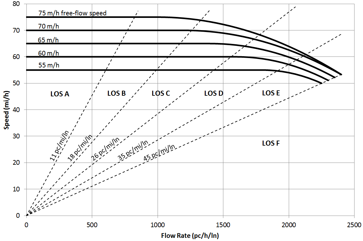
Figure 10.1: HCM Exhibit 12-16

FFS (mi/h)	Capacity (pc/h/ln)
75	2400
70	2400
65	2350
60	2400
55	2300
75	2250

10.6.3 Capacity (Simulation)

For microscopic simulation programs, capacity is typically a function of the specified minimum vehicle entry headway (into the system) and car-following parameters.

• For example, specifying a value of 1.5 seconds for this input will result in a maximum vehicle entry rate of 2400 (3600/1.5) vehicles per hour per lane.
• Once vehicles enter the system, vehicle headways are governed by the car following model, except for lead vehicles.

An issue to be aware of is that while geometric factors such as lane and shoulder width affect the free-flow speed (which in turn affects capacity) in the HCM procedure, some simulation programs do not account for these effects, or they may account for other factors, such as horizontal curvature, that the HCM procedure does not consider.

10.6.4 Lane Distribution (HCM)

For basic freeway segments, there is an implicit assumption that for any given vehicle demand, the vehicles are evenly distributed across all lanes.

For ramp junctions, the HCM procedure includes calculations to determine how vehicles are distributed across lanes as a result of merging or diverging movements.

For weaving segments, there is not an explicit determination of flow rates in specific lanes, but consideration of weaving and non-weaving flows and the number of lanes available for each is an essential element of the analysis procedure.

10.6.5 Lane Distribution (Simulation)

The distribution of vehicles across lanes is typically specified just for the entry points of the network. Once vehicles have entered the network, the vehicles will be distributed across lanes according to car-following and lane-changing logic.

This input value should reflect field data if it is available. If field data indicate an imbalance of flows across lanes, this situation may lead to a difference in results between the HCM and the simulation tool. If field data are not available, specifying an even distribution of traffic across all lanes is probably reasonable for networks that begin with a long length of a basic segment.

If there is a ramp junction within a short distance downstream of the entry point of the network, setting the lane distribution values to be consistent with those from the HCM ramp segment analysis will likely yield more consistent results.

10.6.6 Traffic Stream Composition (HCM)

Vehicles

• The HCM deals, mostly, with the presence of non-passenger car vehicles in the traffic stream by applying passenger car equivalent (PCE) values.
• These values are based on the percentage of small trucks and large trucks in the traffic stream, as well as type of terrain (grade profile and its length).
• Thus, the traffic stream is converted into some equivalent number of only passenger cars, and the analysis results are based on flow rates in these units.

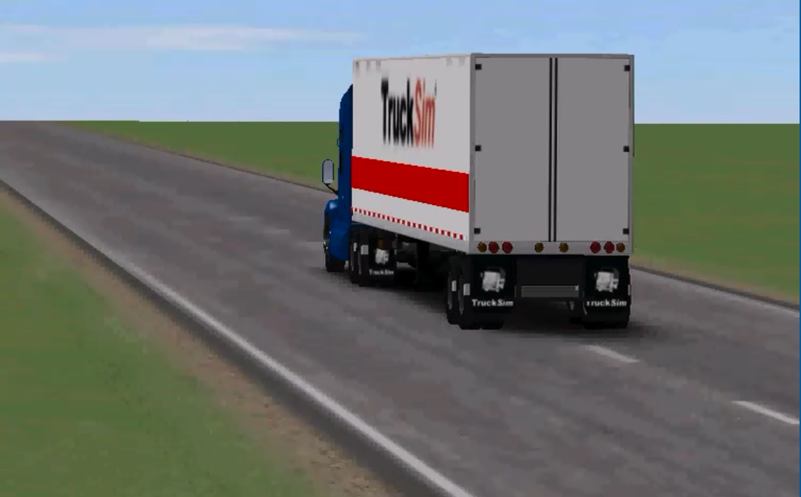
Figure 10.2: Simulation usually explicitly models heavy vehicles

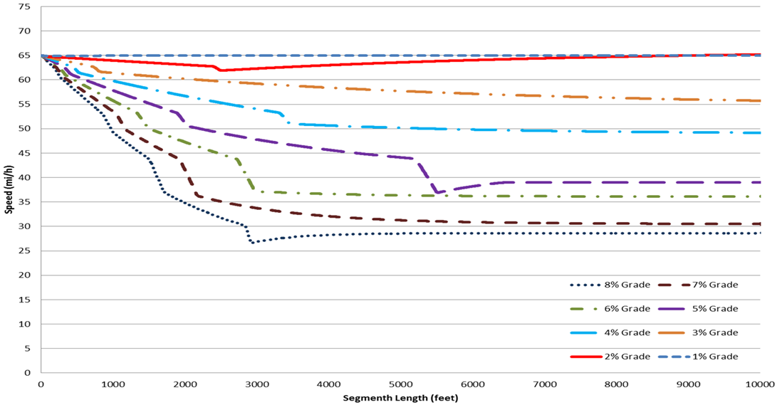
Figure 10.3: Example of impact of trucks on speed for varying upgrades

Drivers

• The HCM procedures do not explicitly account for differences in driver types.
  
• However, the empirical data that the HCM procedures are based on include the effects of the various driver types present in the traffic streams during data collection.

10.6.7 Traffic Stream Composition (Simulation)

Vehicles

• Simulation programs deal with the traffic stream composition just as it specified; that is, the specific percentages of each vehicle type are generated into the system and moved through the system according to their specific vehicle attributes (acceleration, deceleration capabilities, etc.).
  
• Thus, simulation results likely better reflect the effects of non-passenger car vehicles on the traffic stream.
  
• Although in some instances the PCE values contained in the HCM were developed from simulation data, simplifying assumptions made to make them implementable in an analytical procedure result in some loss of fidelity of the treatment of different vehicle types.
• In the case of stochastic-based simulators, the generated vehicle type percentages may only approximate the specified percentages.

Drivers

• Most microscopic simulation programs explicitly provide for a range of driver types and allow a number of factors related to driver type to be modified (e.g., desired speed, gap acceptance threshold, etc.).

10.6.8 Comparison of HCM Results to Simulation Results

10.6.8.1 Density

HCM

• The HCM procedures report density in terms of passenger cars per mile.
• Passenger car equivalency (PCE) factors are used to convert heavy vehicles to passenger cars.
• PCEs are applied prior to the density computations.

Simulation

• Simulation tools report density in terms of actual vehicles per mile.
  
• The effect of heavy vehicles is an explicit result of their different characteristics. Because of this difference, it is difficult to apply PCE factors in reverse to simulation results for purposes of comparison to HCM results.

10.6.8.2 Flow Rate

• The HCM procedures deal with peak 15‐min period demand flow rates, by applying a peak hour factor (PHF) to hourly volumes.
  
• Simulation tools do not normally apply a PHF to input volumes. Some care must therefore be used to ensure that the demand and time periods are represented appropriately to promote the development of comparable results.

10.6.8.3 Ramp Junctions

• The individual segment analysis of ramp merge/diverge segments focus on the density of traffic within the influence of the merge area (usually the ramp and the two adjacent lanes).
  
• The segment length is also assumed to be 1500 ft.
  
• To obtain comparable results from simulation, it is necessary to define the merge area as a separate segment for analysis and to isolate the movements in the adjacent lanes.
• HCM method does not strictly adhere to q = uk relationship

The HCM procedures typically do not consider the effect of self‐aggravating phenomena on the performance of a segment. For example, when traffic in a left turn bay spills over into the adjacent through lane the effect of the through lane performance is not considered. The inability of drivers to access their desired lane when queues back up from a downstream facility is not taken into consideration.

Full numerical compatibility between HCM and simulation‐based analyses will seldom be attainable because of the differences in definitions, modeling approaches, and computational methodologies. For example, differences in the implicit or explicit representation of the network structure may lead to unavoidable differences in a performance measure result, even if all other differences were able to be controlled for between HCM and simulation. One such performance measure is control delay, which by the HCM definition includes delay due to deceleration, stop, and acceleration—these components usually span more than one link in a simulation network, yet the simulation calculation procedures usually do not consider the acceleration delay downstream of the signal stop bar.

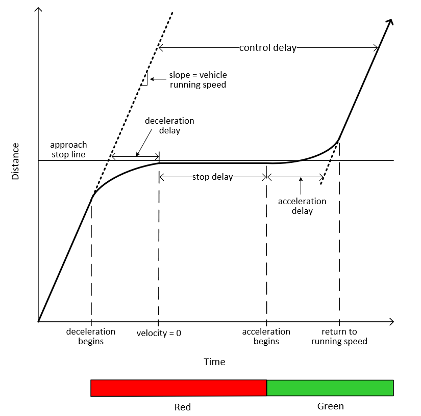
Figure 10.4: Illustration of HCM Control Delay Definition