Chapter 2 Fundamentals of Uninterrupted Traffic Flow and Queuing Theory
2.1 Traffic Stream Parameters
2.1.1 Introduction
Streams of traffic are comprised of individual vehicles, piloted by individual drivers, interacting with each other and the roadway environment (geometry, traffic control devices, etc.).
Because each driver behaves in a unique way (i.e., has its own brain), it is not possible to describe traffic flow as theoretically concisely as other purely physical phenomena. This makes the field of traffic engineering especially challenging.
Nonetheless, we still need ways to quantify traffic streams, so we can analyze and evaluate existing transportation facilities, and design improvements for those facilities.
There are several parameters that we will now discuss that are used to quantitatively describe traffic streams.
2.1.2 Flow Classification
- Two general types of flow environments:
- Uninterrupted flow – traffic flow influenced by characteristics of roadway and interactions of vehicles within the traffic stream
- Interrupted Flow – traffic streams also operate under the influence of traffic control devices
2.1.3 Parameter Classification
- Traffic stream parameters are generally classified in two categories:
- Microscopic - refer to characteristics specific to individual pairs of vehicles within the traffic stream
- Macroscopic - refer to characteristics of the traffic stream as a whole. Represents an aggregation of the microscopic measures.
2.1.4 Microscopic Parameters
- Two commonly used microscopic parameters are:
- Spacing – the physical distance between successive vehicles
- Headway – the time between successive vehicles as they pass a point on a lane or roadway Note that measurements should reference the same point on each vehicle (e.g., front bumper)
- The three main macroscopic parameters that form the underpinning of traffic analysis are:
- Flow, q
- Speed, u
- Density, k
- Flow, q
2.1.5 Flow
Traffic flow is defined as
\[q = \frac{n}{t} \tag{Textbook Eq. 5.1}\]
where:
q = traffic flow in vehicles per unit time,
n = number of vehicles passing some designated roadway point during time t, and
t = duration of time interval.
The time between the passage of successive vehicles, at some designated highway point, is known as the time headway. These time headways are related to t, as defined in Eq. 5.1, by
\[t = \sum_{i\ = \ 1}^{n}h_{i}\tag{Textbook Eq. 5.2}\]
where:
t = duration of time interval,
hi = time headway of the ith vehicle (the time that has transpired between the arrival of vehicle i and i -1), and
n = number of measured vehicle time headways at some designated roadway point.
Substituting Eq. 5.2 into Eq. 5.1 gives
\[q = \frac{n}{\sum_{i\ = \ 1}^{n}h_{i}}\tag{Textbook Eq. 5.3}\]
or
\[q = \frac{1}{\overline{h}}\tag{Textbook Eq. 5.4}\]
where:
\[\overline{h} \text { is the average time headway,}\] \[\frac{\sum h_{i}}{n} \text { in unit time per vehicle.}\]
Typical volume measures:
- Daily Time Unit
- Average Annual Daily Traffic (AADT)
- Total daily volume passing point on roadway in both directions
- Total yearly traffic volume divided by number of days in year
- Total yearly traffic volume divided by number of days in year
- Total daily volume passing point on roadway in both directions
- Average Annual Weekday Traffic (AAWT)
- Average Annual Daily Traffic (AADT)
- Hourly Time Unit
- Peak Hour Volume
Sometimes design peak hour volumes are estimated from daily volume projections, using three parameters:
AADT
K – proportion of daily traffic occurring during the peak hour
D – proportion of peak-hour traffic traveling in the peak direction
Typical range of K and D values:
K: 0.08 – 0.12
D: 0.52 – 0.62 (1.0 for one-way roadway)
- Directional Design Hour Volume (DDHV)
\[DDHV = AADT \times K \times D \tag{Textbook Eq. 6.25}\]
Peak Hour Factor (PHF)
- typically used in traffic analysis methods of HCM
\[PHF = \frac{V}{V_{15} \times 4} \tag{Textbook Eq. 6.8}\]
V = hourly volume for hour of analysis,
V15 = maximum 15-min volume within hour of analysis, and
4 = number of 15-min periods per hour.
2.1.6 Speed
Average traffic speed is defined in two ways:
- Time (spot) mean speed is the average speed of all vehicles passing a point on a roadway over a specified time (instantaneous point speed, as taken by a radar gun for example).
\[{\bar{u}}_{t}\text{ = }\frac{\sum_{i\ = \ 1}^{n}u_{i}}{n}\tag{Textbook Eq 5.5}\]
where:
\({\bar{u}}_{t}\) = time-mean speed in unit distance per unit time,
ui = spot speed (the speed of the vehicle at the designated point on the highway, as might be obtained using a radar gun) of the ith vehicle, and
n = number of measured vehicle spot speeds.
Space mean speed is the average speed of all vehicles occupying a given section of roadway over a specified time (essentially, the inverse of travel time for all vehicles over the specified section length).
This second definition of speed is more useful in the context of traffic analysis and is determined on the basis of the time necessary for a vehicle to travel some known length of roadway.
\[{\bar{u}}_{s} = \frac{l}{\bar{t}}\tag{Textbook Eq. 5.6}\]
where:
\({\bar{u}}_{s}\) = space-mean speed in unit distance per unit time,
l = length of roadway used for travel time measurement of vehicles,
\({\bar{t}}\)= average vehicle travel time, defined as
\[\bar{t} = \frac{1}{n}\sum_{i = 1}^{n}t_{i}\tag{Textbook Eq. 5.7}\]
where:
ti = time necessary for vehicle i to travel roadway section of length l, and n = number of measured vehicle travel times.
Substituting Eq. 5.7 into Eq. 5.6 gives
\[{\bar{u}}_{s} = \frac{l}{\frac{1}{n}\sum_{i = 1}^{n}t_{i}}\tag{Textbook Eq. 5.8}\]
or
\[{\bar{u}}_{s} = \frac{1}{\frac{1}{n}\sum_{i = 1}^{n}\left\lbrack \frac{1}{\left( \frac{l}{t_{i}} \right)} \right\rbrack}\tag{Textbook Eq. 5.9}\]
which is the harmonic mean of speed (space-mean speed). Space-mean speed is the speed parameter used in traffic models.
- Typical Speed Measures
- Average - arithmetic mean (TMS) or harmonic mean (SMS)
- 85th Percentile - speed at which 85% of the vehicles are traveling at or below
- Running - does not include stopped delay
- Average - arithmetic mean (TMS) or harmonic mean (SMS)
2.1.7 Density
Traffic density is defined as
\[k = \frac{n}{l}\tag{Textbook Eq. 5.10}\]
where:
k = traffic density in vehicles per unit distance,
n = number of vehicles occupying some length of roadway at some specified time, and
l = length of roadway.
The density can also be related to the individual spacing between successive vehicles. The roadway length, l, in Eq. 5.10 can be defined as
\[l\ = \sum_{i\ = \ 1}^{n}s_{i}\tag{Textbook Eq. 5.11}\]
where:
si = spacing of the ith vehicle (the distance between vehicle i and i-1, measured from same vehicle reference point), and
n = number of measured vehicle spacings.
Substituting Eq. 5.11 into Eq. 5.10 gives
\[k\ = \frac{n}{\sum_{i\ = \ 1}^{n}s_{i}}\tag{Textbook Eq. 5.12}\]
\[k\ = \frac{1}{\bar{s}}\tag{Textbook Eq. 5.13}\]
where:
\[\overline{s} \text { is the average vehicle spacing,}\] \[\frac{\sum s_{i}}{n} \text { in unit distance per vehicle.}\]
2.1.8 Variable Relationships
Based on the definitions presented above, a simple identity provides the basic relationship among traffic flow, speed (space-mean speed), and density (denoting space-mean speed, \({\bar{u}}_{s}\), as simply u for notational convenience),
\[q = u \times k\tag{Textbook Eq. 5.14}\]
where:
q = flow, typically in units of vehicles per hour (veh/h),
u = speed (space mean speed), typically in units of mi/h, and
k = density, typically in units of veh/mi.
2.1.9 Basic Traffic Stream Models: Speed vs. Density
\[u = u_{f}\left(1 - \frac{k}{k_{j}} \right)\tag{Textbook Eq. 5.15}\]
where:
u = space-mean speed in mi/h,
uf = free-flow speed in mi/h,
k = density in veh/mi, and
kj = jam density in veh/mi.
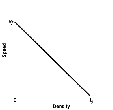
Figure 2.1: Speed-Density relationship (source: Textbook Fig. 5.1)
2.1.10 Basic Traffic Stream Models: Flow vs. Density
\[q = u_{f}\left(k - \frac{k^{2}}{k_{j}} \right)\tag{Textbook Eq. 5.16}\]
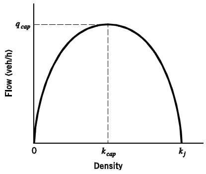
Figure 2.2: Flow-Density relationship (source: Textbook Fig. 5.2)
2.2 Models of Traffic Flow
2.2.1 Introduction
- Macroscopic relationships and analyses are very valuable, but
- A considerable amount of traffic analysis occurs at the microscopic level
- In particular, we often are interested in the elapsed time between the arrival of successive vehicles (i.e., time headway)
- Essential to queuing analysis
2.2.3 Uniform
- The simplest approach to modeling vehicle arrivals is to assume a uniform spacing
- This results in a deterministic, uniform arrival pattern—in other words, there is a constant time headway between all vehicles
- However, this assumption is usually unrealistic, as vehicle arrivals often follow a stochastic process
- Thus, a model that represents a random arrival process is usually needed
2.2.4 Poisson
- Discrete distribution
- Commonly referred to as ‘counting distribution’
- Represents the count distribution of random events
For a sequence of events to be considered truly random, two conditions must be met:
- Any point in time is as likely as any other for an event to occur (e.g., vehicle arrival)
- The occurrence of an event does not affect the probability of the occurrence of another event (e.g., the arrival of one vehicle at a point in time does not affect the arrival time of any other vehicle)
The p.m.f. equation for the Poisson distribution is:
\[P(n) = \frac{\left({\lambda t} \right)^{n}e^{-{\lambda t}}}{n!}\tag{Textbook Eq. 5.23}\]
p(n) = probability of exactly n vehicles arriving in a time interval t
n = # of vehicles arriving in a specific time interval
λ = average rate of arrival (veh/unit time)
t = selected time interval (duration of each counting period (unit time))
The p.m.f. is also commonly expressed as:
\[P(n) = \frac{\left({m} \right)^{n}e^{-{m}}}{n!}\]
p(n) = probability of exactly n vehicles arriving in a time interval t
n = number of vehicles arriving in a specific time interval
m = average number of occurrences during a specific time period t (i.e., m = λt)
2.2.5 Negative Exponential
The assumption of Poisson distributed vehicle arrivals also implies a distribution of the time intervals between the arrivals of successive vehicles (i.e., time headway).
To demonstrate this, let the average arrival rate, λ, be in units of vehicles per second, so that
\[\lambda\ = \frac{q}{3600}\frac{\text{veh/h}}{\text {s/h}}=\frac{\text{veh}}{\text{s}}\tag{Textbook Eq. 5.24}\]
Substituting into the Poisson equation yields
\[P\left( n \right)\ = \frac{\left( \frac{{qt}}{3600} \right)^{n} \times e^{- \frac{{qt}}{3600}}}{n!}\tag{Textbook Eq. 5.25}\]
Note that the probability of having no vehicles arrive in a time interval of length t (P(0)) is the equivalent of the probability of a vehicle headway, h, being greater than or equal to the time interval t.
So from the previous equation,
\[P\left(0 \right)\ = P\left( h \geq t \right)\tag{Textbook Eq. 5.26}\]
\[\frac{(1)e^{\frac{-qt}{3600}}}{1} = e^{\frac{-qt}{3600}}\]
Note: x0 = 1, 0! = 1
This distribution of vehicle headways is known as the negative exponential distribution.
2.3 Freeway Queuing
2.3.1 Introduction
The purpose of traffic queuing models is to provide a means to estimate important measures of freeway performance, including vehicle delay and traffic queue lengths. Such estimates are critical to roadway design (the required length of left-turn bays and the number of lanes at intersections) and traffic operations control, including the timing of traffic signals at intersections.
Queuing models are often identified by three alphanumeric values. The first value indicates the arrival rate assumption, the second value gives the departure rate assumption, and the third value indicates the number of departure channels. For traffic arrival and departure assumptions, the uniform, deterministic distribution is denoted D and the stochastic, exponential distribution is denoted M. Thus a D/D/1 queuing model assumes deterministic arrivals and departures with one departure channel. Similarly, an M/D/1 queuing model assumes exponentially distributed arrival times, deterministic departure times, and one departure channel.
The case of deterministic arrivals and departures with one departure channel (D/D/1 queue) is an excellent starting point in understanding queuing models because of its simplicity. The D/D/1 queue lends itself to an intuitive graphical or mathematical solution, which will be illustrated by an in-class example.
2.3.2 Traffic Analysis at Freeway Bottlenecks
Some of the most severe congestion problems occur at freeway bottlenecks, which are defined as a portion of freeway with a lower capacity (qcap) than the incoming section of freeway. This reduction in capacity can originate from a number of sources, including a decrease in the number of freeway lanes and reduced shoulder widths (which tend to cause drivers to slow and thus effectively reduce freeway capacity).
There are two general types of traffic bottlenecks—those that are recurring and those that are incident induced. Recurring bottlenecks exist where the freeway itself limits capacity—for example, by a physical reduction in the number of lanes. Traffic congestion at such bottlenecks results from recurring traffic flows that exceed the vehicle capacity of the freeway in the bottleneck area. In contrast, incident-induced bottlenecks occur as a result of vehicle breakdowns or accidents that effectively reduce freeway capacity by restricting the through movement of traffic. Because incident-induced bottlenecks are unanticipated and temporary in nature, they have features that distinguish them from recurring bottlenecks, such as the possibility that the capacity resulting from an incident-induced bottleneck may change over time. For example, an accident may initially stop traffic flow completely, but as the wreckage is cleared, partial capacity (one lane open) may be provided for a period of time before full capacity is eventually restored. A feature shared by recurring and incident-induced bottlenecks is the adjustment in traffic flow that may occur as travelers choose other routes and/or different trip departure times, to avoid the bottleneck area, in response to visual information or traffic advisories.
The most intuitive approach to analyzing traffic congestion at bottlenecks is to assume D/D/1 queuing, which will be illustrated by an in-class example.