Chapter 7 HCM Freeway Facility

7.1 Undersaturated Analysis

7.1.1 Overview

The analysis methodology is used for conducting larger freeway analyses from a combination of the three freeway components:

• Basic segments, merge/diverge segments, and weaving segments.

It can analyze multiple contiguous segments over multiple time intervals.

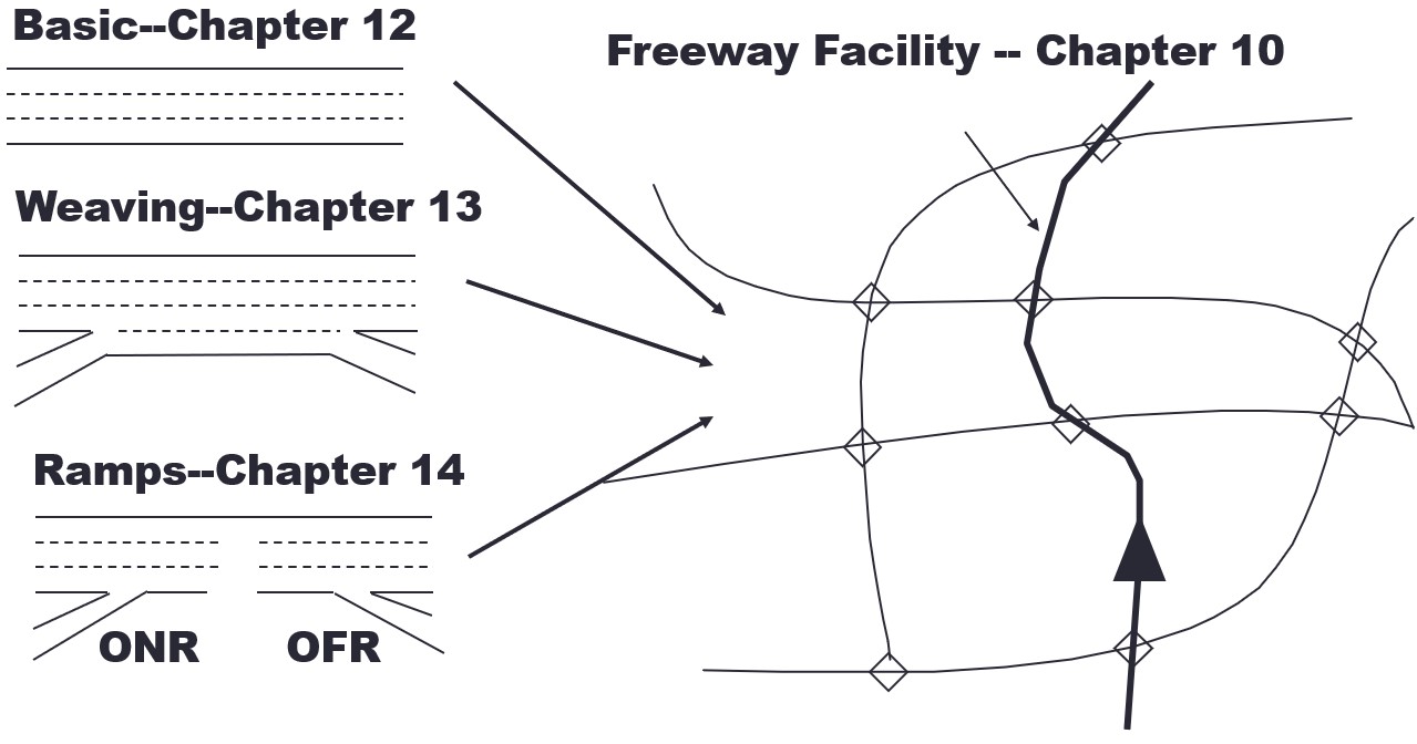
Figure 7.1: HCM Freeyway Facility Undersaturated

7.1.2 Analysis Procedure

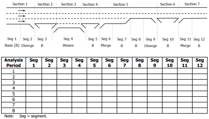
• Divide the facility into segments
• Set number of time periods
  • The default time period duration is 15 minutes
  • Thus, a 1-hour analysis duration would use 4 time periods
• Calculate demand analysis flow rates
  • Even though the time period duration is 15 minutes, the analysis flow rates are entered as hourly volumes
• Determine segment capacities from Chaps. 12, 13, and 14
• Determine inputs for required for each individual segment analysis procedure (i.e., FFS, demand, %HV, etc.)
• Calculate d/c ratio for each segment and time period
• For undersaturated facility:
  • Calculate density for each segment
  • Determine LOS for each segment
  • Calculate density for entire facility
  • Determine LOS for entire facility
  • Other performance measures can be calculated as needed

7.1.3 Facility Segmentation

Figure 7.2: Freeway Segmentation

7.1.4 Time-Space Domain of Freeway Facility

Figure 7.3: Time-Space Matrix

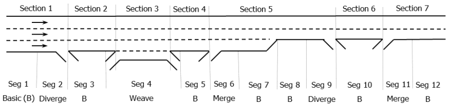
7.1.5 Facility Segmentation Considerations

Merge/Diverge (Ramp) Segments

• Default length of a ramp segment is 1500 ft.

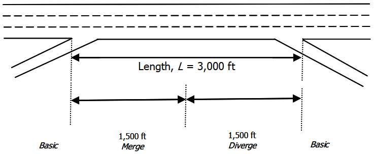
Figure 7.4: Ramp Segmentation 1

• If there is more than 3000 ft between ramps, place a basic segment in between.
  • The length of the basic segment will be the total separation distance between the ramps minus 3000 ft.

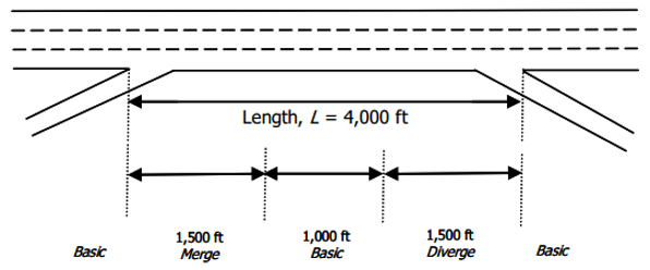
Figure 7.5: Ramp Segmentation 2

• If there is less than 3000 ft between ramps, place an ‘overlap’ segment in between
  • The length of the overlap segment will be 3000 ft minus the total separation distance between the ramps.

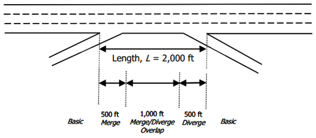
Figure 7.6: Ramp Segmentation 3

• If a lane is added at an on-ramp junction (i.e., the “acceleration lane” is a full lane), the ramp segment is analyzed as a basic segment.
  
• If a lane is dropped at an off-ramp junction (i.e., the outer lane turns into the off-ramp lane), the ramp segment is analyzed as a basic segment.

Weaving Segments

• If the short length is greater than L_max, the weaving segment is analyzed as a basic segment.

7.1.6 Demand Flow Rates

• Determine demands by time period (default is 15 min)
  
• Ensure that the sum of inputs equals the sum of outputs
  
• Adjust flow rates for heavy vehicles
  
• The PHF is not used since the time period duration is 15 minutes

7.1.7 Segment Capacity Estimation and Adjustment

Determine segment capacities according to the methods of Chapters 12, 13, and 14.

• Segment adjustments
  • Construction activities or work zones
  • Adverse weather (rain, snow, fog)
  • Incidents or accidents

Ramp metering can be accommodated by modifying on-ramp roadway capacities.

7.1.8 Compute d/c Ratios

Calculate demand/capacity ratio for each segment for each time period

If all segment d/c ratios are \(\leq\) 1.0 for a time period, then segment performance measures are calculated according to Chapters 12, 13, and/or 14.

If any segment d/c ratio > 1.0 in a given time period, then the oversaturated analysis module is applied for all facility segments during that time period and subsequent time periods until the congestion clears.

7.1.9 Downstream Speed Constraint

In case of a slow average speed for a segment upstream of the subject segment, the subject segment speed will be constrained, per Eq. 25-1.

\[V_{max} = FFS - \left( FFS - v_{prev} \right) \times e^{-0.00162 \times L}\]

where:

\(V_{max}\) = maximum achievable segment speed (mi/h),
FFS = segment free-flow speed (mi/h),
\(V_{prev}\) = average speed on immediate upstream segment (mi/h), and
L = distance from midpoints of the upstream segment and the subject segment (ft).

7.1.10 Density

Segment densities are calculated per the methods of chapters 12, 13, and 14. However, merge/diverge segments use density for entire cross-section.

Facility density is calculated per Eq. 10-1.

\[D_{Fwy} = \frac{\sum_{i = 1}^{n}{D_{i} \times L_{i} \times N_{i}}}{\sum_{i = 1}^{n}{L_{i} \times N_{i}}}\]

where:

\(D_{Fwy}\) = average density for the facility in a given 15-min analysis period (pc/mi/ln),
\(D_{i}\) = density for segment i (pc/mi/ln),
\(L_{i}\) = length of segment i (miles),
\(N_{i}\) = number of lanes in segment i, and
n = number of segments in the defined facility.

7.1.11 LOS

Segment LOS is determined per chapters 12, 13, and 14.

Facility LOS is determined per Exhibit 10-6. Note that the LOS criteria for urban areas are the same as for basic segments.

Level of Service	Urban	Rural
A	\(\leq\) 11	\(\leq\) 6
B	> 11-18	> 6-14
C	> 18-26	> 14-22
D	> 26-35	> 22-29
E	> 35-45	> 29-39
F	> 45 or Demand exceeds capacity	> 39 or Demand exceeds capacity

For more information on rural area thresholds, see:

• Washburn, Scott S. and Kirschner, David S. Rural Freeway Level of Service Based Upon Traveler Perceptions. Transportation Research Record: Journal of the Transportation Research Board. No. 1998, Transportation Research Board of the National Academies, Washington, D.C., 2006, pp. 31-37. DOI: 10.3141/1988-06

7.1.12 Other Measures Reported

• Volume/Capacity
  
• Demand/Capacity
  
• Average Speed/Travel Time
  
• Free-Flow Travel Time
  
• Delay
  • Mainline, System (includes on-ramp)
    
• veh-mi of travel (VMT)
  
• veh-h of travel (VHT)
  
• veh-h of delay (VHD)

7.1.13 Supporting Calculations (Segment)

\[{TravTim}e_{FF} = \frac{Length}{{Speed}_{FF}}\]

\[{TravTim}e_{Avg} = \frac{Length}{Speed_{Avg}}\]

\[Delay = TravTime_{Avg} - TravTime_{FF}\]

\[VMT = V \times TimePeriodDuration \times Length\]

\[VHT = V \times TimePeriodDuration \times TravTime_{Avg}\]

\[VHD = \left({TravTim}e_{Avg} - TravTime_{FF} \right) \times V \times TimePeriodDuration\]

with:

• V in veh/h
  
• TimePeriodDuration in Hours (default is 0.25; i.e., 15 min)
  
• Length in miles
  
• \(TravTime_{FF}\) in hours
  
• \(TravTime_{Avg}\) in hours
  
• \(Speed_{FF}\) in mi/h
  
• \(Speed_{Avg}\) in mi/h

7.1.14 Supporting Calculations (Facility)

\[{TravTime}_{Avg-Fwy} = \sum_{Seg=1}^{n}{TravTime}_{Avg-Seg}\]

\[{TravTime}_{FF-Fwy} = \sum_{Seg=1}^{n}{TravTime}_{FF-Seg}\]

\[{Speed}_{Avg-Fwy}=\frac{{Length}_{{Fwy}}}{{TravTime}_{Avg-Fwy}}\]

or

\[{Speed}_{Avg-Fwy}=\frac{{VMT}_{Fwy}}{{VHT}_{Fwy}}\]

Other facility measures are summation of segment measures

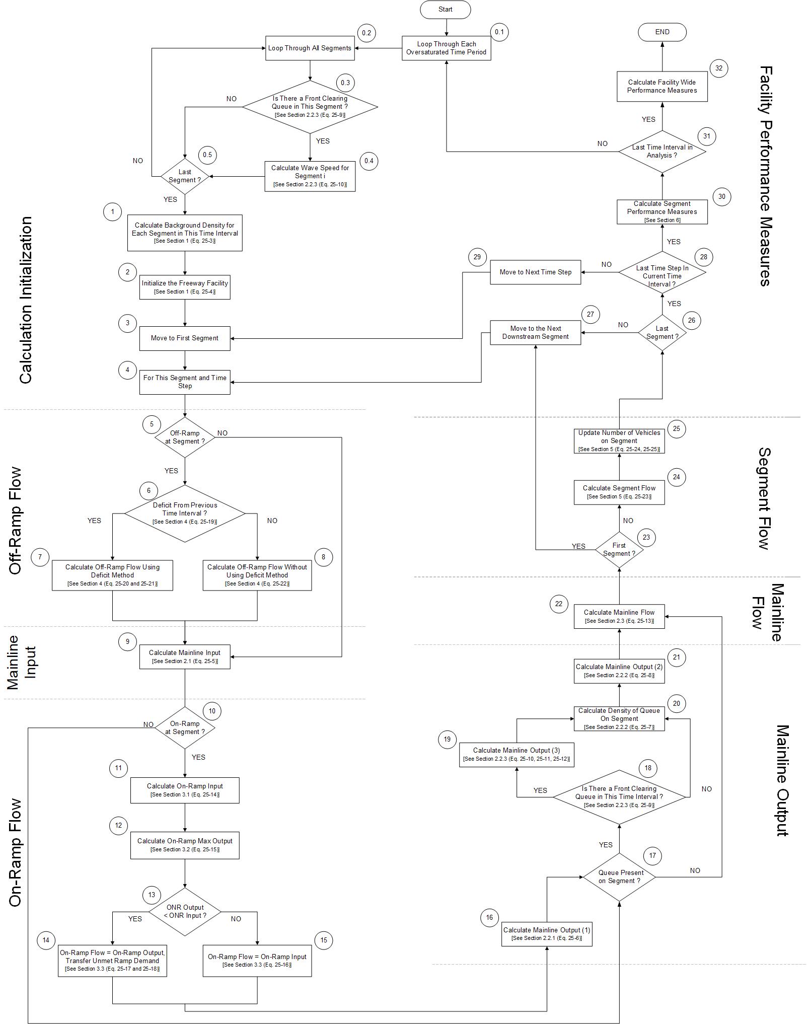
7.2 Oversaturated Analysis

7.2.1 Compute d/c Ratios

If any segment d/c ratio > 1.0 in a given time period, then the oversaturated analysis module is applied for all facility segments in that and subsequent time periods until congestion clears.

7.2.2 Freeway Facility Oversaturated Analysis Methodology Capabilities

• Can account for oversaturation, both spatially and temporally, under certain conditions
  
• Can account for time-varying demand and capacity
  
• Accounts for all active and hidden mainline bottlenecks
  
• Can track queues as they form and dissipate across segments and time intervals
  
• Can represent the effect of short term incidents and work zone effects if properly calibrated

7.2.3 General Limitations of Methodology

• Facility length should be limited to 9-12 mi
  • Traffic will enter and exit freeway in same time interval
• No congestion at start/end of the analysis
• No congestion on first or last segment
• Overlapping bottlenecks cannot be handled
• Off-ramp queue spillback not considered
• On-ramp queuing tracked, but effects upstream of on-ramp not considered

7.2.4 Additional Considerations

• Jam density (pc/mi/ln)
• Post-breakdown maximum flow rate
  • General consensus is that maximum flow rate discharging from a queue (i.e., “discharge flow rate”) is less than pre-breakdown capacity flow rate
  • No consensus on how much reduction; Literature reports general range of 5-15%
  • For HCM, we chose default value of 7% (essentially split the difference)
• Calculations are made in very short discrete time steps
  • 4 time steps per minute; 60 per 15-min time period

7.2.5 Time-Space Domain

In addition to tracking queue formation and dissipation at active bottlenecks, the oversaturation analysis method has the capability to properly account for hidden bottlenecks. A dynamic illustration of the following figure will be demonstrated in class.

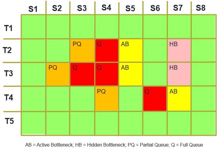
Figure 7.7: Time-Space Matrix

7.2.6 Key Analysis Concepts

Shock Waves

Shock waves occur at points where there is a change in traffic stream characteristics (e.g., densities). For example,

• Faster vehicles catching up to slower vehicles in a school or work zone
  
• Free-flowing vehicles approaching the back of queued vehicles at a bottleneck
  
• Queued vehicles discharging from a signalized intersection approach

A “wave” of changing density will propagate upstream or downstream, depending on specific characteristics of colliding traffic streams.

Demand volume (in units of lanes) for 4 time periods is:
1) 1.5 (< 2 lanes of bottleneck segment, so no queuing)
2) 2.5 (> 2 lanes of bottleneck segment, so backward forming shock wave)
3) 2.0 (= lanes of bottleneck segment, so rear stationary shock wave)
4) 1.5 (< 2 lanes of bottleneck segment, so forward recovery shock wave)

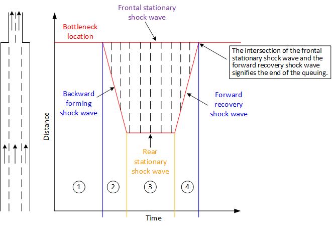
Figure 7.8: Shockwave Diagram

Analysis Time Units

• Minutes per Time Period (min/period) = 15
  
• Time Steps (ts) per Minute (ts/min) = 4
  
• Seconds per Time Step (s/ts) = 60 (s/min) / 4 (ts/min) = 15
  
• Time Steps per Hour (ts/h) = 4 ts/min \(\times\) 60 min/h = 240

Flow-Density Relationship

• Traffic operations in the congested flow regime are not well understood
  
• Given the lack of consensus on appropriate models for describing speed-flow-density relationships for congested flow, the HCM freeway facilities procedure uses a simplified linear relationship to describe congested operations:

\[k_{queue}=k_{cap}+\frac{(k_{jam}-k_{cap})}{q_{cap}} \times (q_{cap}-q)\]

where:

\(k_{queue}\) = density in the queue (veh/mi)
\(k_{cap}\) = density at capacity (veh/mi)
\(k_{jam}\) = jam density (veh/mi)
q = segment flow rate (veh/h)
\(q_{cap}\) = segment capacity flow rate (veh/h)

The speed of the traffic stream in the queue is given by:

\[S_{B}=\frac{S_{O}C_{B}}{C_{B}+S_{O}K_{j}\times \bigg (1-\frac{C_{B}}{C_{N}}\bigg)}\]

where:

\(S_{B}\) = speed of traffic in bottleneck queue (mi/h)
\(S_{O}\) = speed of traffic at capacity flow rate (mi/h); sometimes referred to as ‘optimal speed’
\(C_{B}\) = bottlenenck capacity (veh/h/ln)
\(C_{N}\) = pre-breakdown capacity flow rate (veh/h/ln); sometimes referred to as ‘normal capacity’
\(k_{j}\) = jam density (veh/mi/ln)

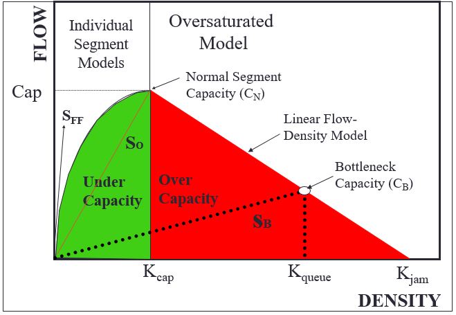
Figure 7.9: Flow Density Relationship

Background Density (KB)

Background density (veh/mi) over Time Period (p) is the density of the subject segment assuming there is no queuing on the segment.

This density is calculated using the expected demand on the segment in the corresponding undersaturated procedure in Chapters 12–14.

\[KB = \frac{v}{S}\]

where:

v = flow rate (veh/h)
S = average speed (mi/h)

Queue Density (KQ)

Queue density on the subject segment during the given time step is calculated on the basis of a linear density‐flow relationship in the congested regime (see Fig. 7.9). Note that the following equation is equivalent to the \(k_{queue}\) equation given above.

\[KQ=KJ-\frac{(KJ-KC) \times SF}{SC}\tag{HCM Eq. 25-10}\]

where:

KJ = jam density (veh/mi/ln)
KC = density at capacity (veh/mi/ln)
SF = segment flow rate (veh/unit time)
SC = segment capacity flow rate (veh/unit time)

On-Ramp Considerations

For an on-ramp, the demand served is a function of the ramp demand and the available capacity on the mainline. If the available capacity, which is the difference between the capacity of the mainline and the upstream mainline demand, is less than one half of a mainline lane of capacity (in the example shown below, this is 5 veh/time step), then you can serve a maximum of one-half of the lane capacity from the on-ramp (5 veh/ts in the example below). Of course, if the ramp demand is less than this value, then just this lower ramp demand value is served. However, the ramp demand also needs to consider unserved (i.e., queued) vehicles from previous time steps.

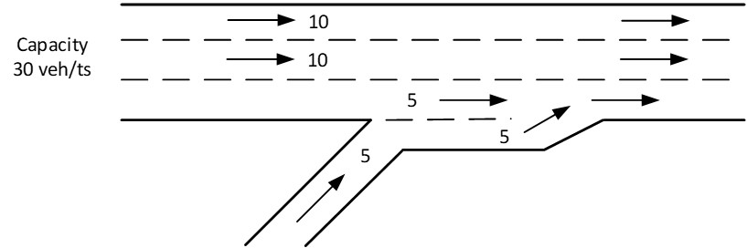
Figure 7.10: On-Ramp Considerations for Oversaturated Analysis

Off-Ramp Considerations

For an off-ramp, we must consider potential demand deficit, which is the amount of unserved traffic from the previous time period. This typically occurs due to a bottleneck immediately upstream of the off-ramp (such as illustrated in the figure below).

When the deficit is greater than the mainline/segment flow, we apply the off-ramp proportion from the previous time period. This is because the deficit traffic is the unserved traffic from the previous time period. The deficit is reduced by the amount of mainline flow per time step.

If the deficit is less than the mainline/segment flow, but greater than zero, then the off-ramp proportion from the previous time period is applied to the deficit amount (again, because this is the left over traffic from the previous time period) and the current time period off-ramp proportion is applied to the difference between the mainline/segment flow and the deficit.

When the deficit is zero, only the off-ramp proportion for the current time period is applied.

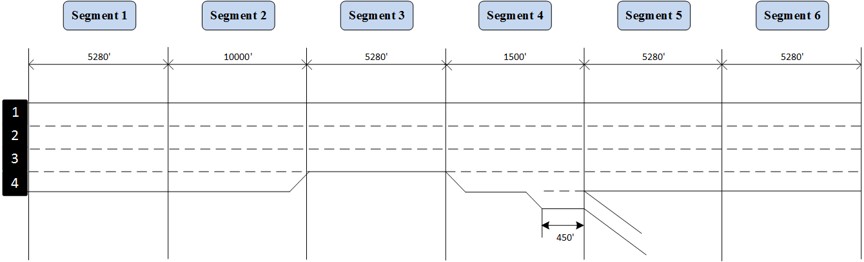
Figure 7.11: Off-Ramp Considerations for Oversaturated Analysis

7.2.7 Methodology Flow Chart

The overall flow of the oversaturation analysis procedure is illustrated in the following flow chart.

Figure 7.12: Oversaturated Analysis Flow Chart

7.3 Travel Time Reliability

7.3.1 Overview

Paraphrased from the Highway Capacity Manual…

• Freeway travel time reliability (TTR) reflects the distribution of the travel times for trips traversing an entire freeway facility over an extended period of time, typically one year, during any portion of the day.
  
• A one-year Reliability Reporting Period (RRP) is typical, as it covers most variation in travel times arising from various factors. Shorter RRPs are possible for special circumstances, such as a focus on summer tourist travel or the work zone construction season.

Rather than evaluating only an ”average” or ”typical” day with good weather and no incidents, a reliability analysis looks at the effects of various conditions/situations that temporarily reduce a freeway’s performance over the course of a year or other long-term time frame, such as…

• Fluctuating demand
  
• Non-ideal weather
  
• Incidents
  
• Work zones

Each combination of demand level, weather condition, incident type, etc. during a given day is termed a ”scenario”.

A set of scenarios is generated (in a software tool) based on the probability of a particular condition occurring; one scenario is generated for each day within the RRP (for example, each non-holiday weekday throughout the year).

The facility travel time is evaluated for each 15-minute time period within the study period for each scenario, by repeatedly applying the Chapter 10 analysis method, resulting in a distribution of travel times that can be used to generate a variety of useful reliability-related performance measures (such as illustrated in the following figure).

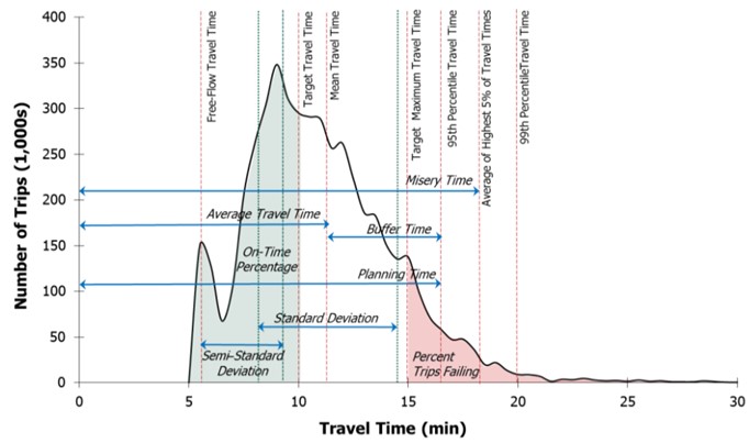
Figure 7.13: Example Travel Time Distribution (Source: Highway Capacity Manual, Chapter 11, 6th Ed.)

The typical analysis units for a TTR analysis are illustrated in the following figure.

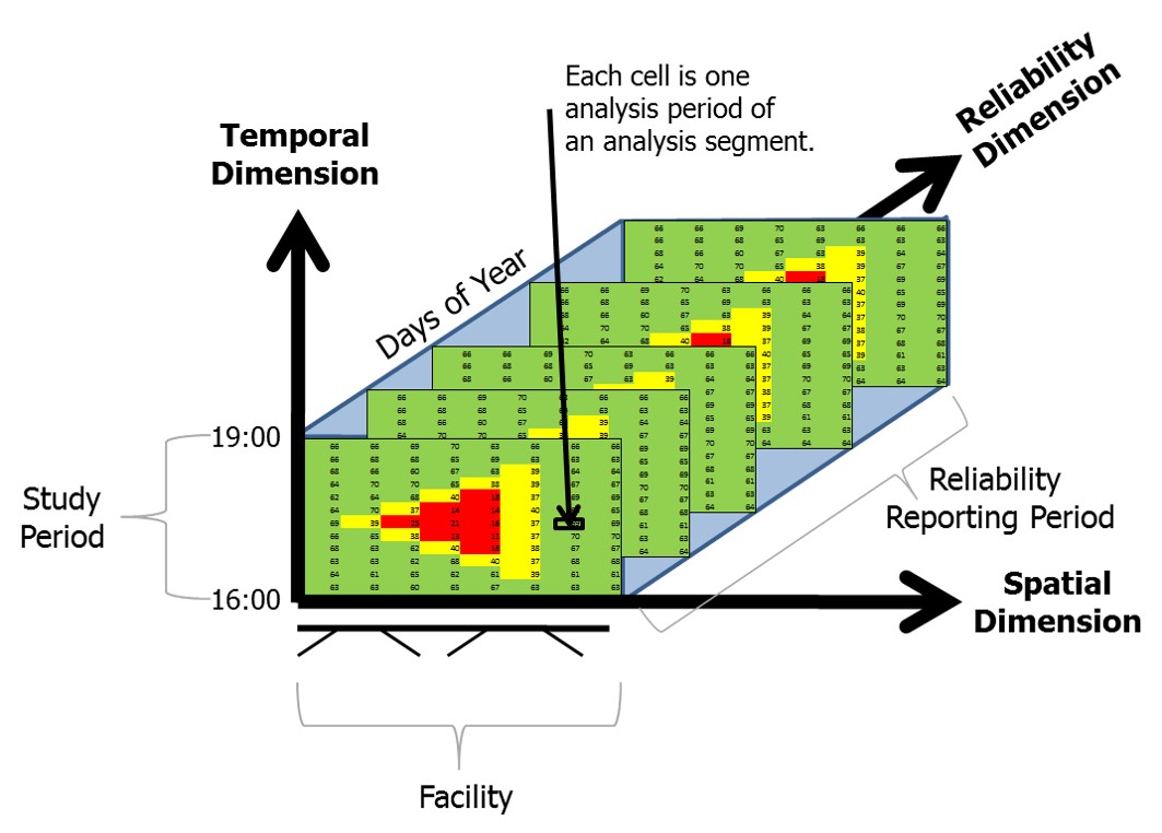
Figure 7.14: Example TTR Analysis Units (Source: Highway Capacity Manual, Chapter 11, 6th Ed.)

A variety of travel time indices are typically used to characterize the results of a TTR analysis.

Travel time index (TTI) is defined as the ratio of the actual travel time to the free-flow travel time. By definition, TTI is always \(\geq\) 1.0.

Percentile travel time index (\(TTI_{pp}\)). Represents the percentile TTI in the travel time distribution. For example…

• \(TTI_{85}\) means that this observation is exceeded only 15% of the time in the travel time distribution.
  
• \(TTI_{50}\) is the median TTI.
  
• \(TTI_{95}\) is the 95th percentile TTI, and is commonly referred to as the planning time index (PTI). Essentially, this is the additional time you should plan for your trip to ensure that you arrive on time all but about once per month (1 out of 20 weekdays).

7.4 References

Transportation Research Board (2022). Highway Capacity Manual, 7th Edition: A Guide for Multimodal Mobility Analysis. Transportation Research Board, Washington, DC. https://nap.nationalacademies.org/catalog/26432/highway-capacity-manual-7th-edition-a-guide-for-multimodal-mobility