4 Example Problem 2
4.1 Passing Constrained Segment with Horizontal Curves
This example problem illustrates the computation of LOS in a single direction of a curving, 0.75-mi-long Passing Constrained segment in level terrain.
The Facts
The segment to be evaluated has the same general demand and geometric characteristics as the segment evaluated in Example Problem 1. The difference is that this segment has horizontal curvature instead of being straight; otherwise, the same inputs are used as for Example Problem 1.
The segment is split into 11 subsegments, with each subsegment being either straight (tangent) or curved. Horizontal curvature data for each subsegment is provided in Exhibit 1.
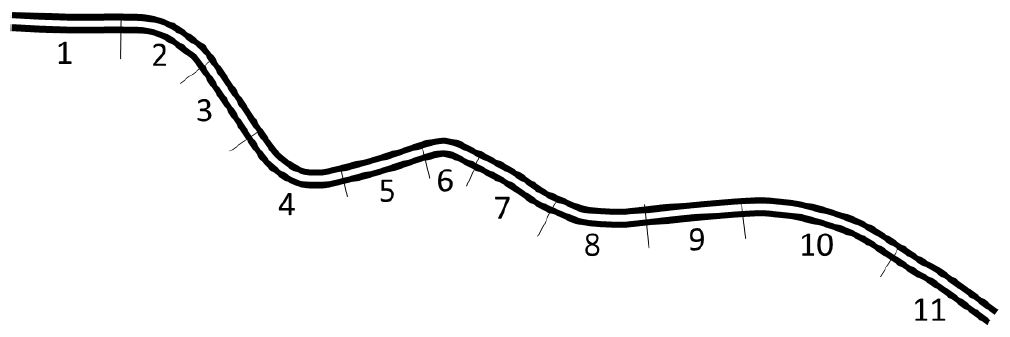
Figure 4.1: Example 2 Highway Segment
| Subsegment | Type | Length (ft)a | Super-elevation (%) | Radius (ft) | Central Angle (deg) | Horizontal Classb |
|---|---|---|---|---|---|---|
| 1 | Tangent | 280 | – | – | – | – |
| 2 | Horizontal curve | 432 | 3 | 450 | 55 | 3 |
| 3 | Tangent | 260 | – | – | – | – |
| 4 | Horizontal curve | 366.5 | 2 | 300 | 70 | 4 |
| 5 | Tangent | 250 | – | – | – | – |
| 6 | Horizontal curve | 216 | 5 | 275 | 45 | 5 |
| 7 | Tangent | 275.6 | – | – | – | – |
| 8 | Horizontal curve | 458 | 0 | 750 | 35 | 2 |
| 9 | Tangent | 285 | – | – | – | – |
| 10 | Horizontal curve | 767.9 | 4 | 1,100 | 40 | 1 |
| 11 | Tangent | 369 | – | – | – | – |
| Total | 3,960 |
a Length for horizontal curves = radius × central angle × π/180.
b Determined from Exhibit 15-22, with radius and superelevation as inputs.
Objective
Estimate the average speed in the subject direction on the two-lane highway taking into account the effects of horizontal alignment on the average speed.
Step 1: Identify Facility Study Boundaries and Segmentation
This step was completed in Example Problem 1. The horizontal alignment does not affect the selection of study boundaries and segmentation.
Step 2: Determine Demand Flow Rates, Capacity, and d/c Ratio
This step was completed in Example Problem 1. The horizontal alignment does not affect the computation of the demand flow rates.
Step 3: Determine the Vertical Alignment Classification
This step was completed in Example Problem 1. The horizontal alignment does not affect the determination of the vertical alignment classification.
Step 4: Determine the Free-Flow Speed
This step was completed in Example Problem 1. The computed base FFS applies to the tangent subsegments.
Step 5: Estimate the Average Speed
Steps 5a, 5b, and 5c were applied in Example Problem 1 to obtain the following speed results for the tangent subsegments:
Base free-flow speed BFFS = 57.0 mi/h,
Tangent free-flow speed FFS = 56.8 mi/h, and
Average speed for tangent subsegments S = 53.7 mi/h.
Step 5d: Adjust Speed for Horizontal Alignment
In this step, the average speed for each subsegment with a horizontal curve is determined. There are three substeps: (a) identifying the horizontal alignment classification for each subsegment with a horizontal curve, (b) calculating the average speed for each subsegment with a horizontal curve, and (c) calculating the adjusted average speed for the segment.
Step 5d.1: Identify all Horizontal Curves Within the Segment
In this step the tangent (straight) length, curve radius, and superelevation are identified for each horizontal curve within the segment. Each curve is assigned a horizontal alignment classification on the basis of its radius and percent superelevation, using Exhibit 15-22. The resulting horizontal classes were indicated previously in Exhibit 1. Note that in typical designs, the crown of the roadway (designed to shed water from the paved way) will cause the superelevation to vary by direction of travel. Therefore, a curve’s horizontal class may also vary by direction of travel.
Step 5d.2: Calculate Average Speed for each Horizontal Curve Within the Segment
The average speed for a subsegment with horizontal curvature is determined using Equation 15-12 though Equation 15-15. The process is demonstrated for Subsegment 2.
Subsegment 2 has a horizontal alignment class of 3 and the BFFS for the preceding tangent section is 57.0 mi/h. Equation 15-14 is applied to compute the base free-flow speed for Subsegment 2:
\[{BFFS}_{{HC}2} = \text{min}\left( {BFFS}_{T},44.32 + 0.3728 \times {BFFS}_{T} - 6.868 \times {HorizClass}_{2} \right)\]
\[{BFFS}_{{HC}2} = \text{min}(57.0,\ 44.32 + 0.3728 \times 57.0 - 6.868 \times 3)\]
\[{BFFS}_{{HC}2} = \text{min}(57.0,\ 44.9656) = 44.9656\ \text{mi/h}\]
Subsegment 2’s FFS is computed using Equation 15-13:
\[{FFS}_{HC2} = {BFFS}_{HC2} - 0.0255 \times HV\%\]
\[{FFS}_{HC2} = 44.9656 - 0.0255 \times 5\]
\[{FFS}_{HC2} = 44.8381\ \text{mi/h} \]
The slope coefficient m used in the determination of average speed is computed using Equation 15-15 as follows:
\[m = \text{max}\left( 0.277, - 25.8993 - 0.7756 \times {FFS}_{HC2} + 10.6294 \times \sqrt{{FFS}_{HC2}} + 2.4766 \times {HorizClass}_{2} \\ - 9.8238 \times \sqrt{{HorizClass}_{2}} \right)\]
\[m = \text{max}\left( 0.277, - 25.8993 - 0.7756 \times 44.8381 + 10.6294 \times \sqrt{44.8381} + 2.4766 \times 3 \\ - 9.8238 \times \sqrt{3} \right)\]
\[m = \text{max}(0.277,\ 0.9145) = 0.9145\]
Finally, the average speed of Subsegment 2 is computed by Equation 15-12.
\[S_{{HC}2} = \text{min}\left( S,{FFS}_{{HC}2} - m \times \sqrt{\frac{v_{d}}{1,000} - 0.1} \right)\]
\[S_{{HC}2} = \text{min}\left( 53.7,\ 44.8381 - 0.9145 \times \sqrt{\frac{800}{1,000} - 0.1} \right)\]
\[S_{{HC}2} = \text{min}(53.7,\ 44.0730) = 44.1\ \text{mi/h}\]
Similar computations are performed for the other subsegments with horizontal curves. The results are presented in Exhibit 26-19.
| Subsegment | BFFSHci (mi/h) | FFSHci (mi/h) | m | SHci (mi/h) |
|---|---|---|---|---|
| 2 | 44.9656 | 44.8381 | 0.9145 | 44.1 |
| 4 | 38.0976 | 37.9701 | 0.4081 | 37.6 |
| 6 | 31.2296 | 31.1021 | 0.2770 | 30.9 |
| 8 | 51.8336 | 51.7061 | 1.4905 | 50.5 |
| 10 | 57.0000 | 56.8725 | 2.8036 | 53.7 |
Step 5d.3: Calculate Adjusted Average Speed for the Segment
The speed results for all subsegments are summarized in Exhibit 26-20.
| Subsegment | Type | Speed (mi/h) | Length (ft) |
|---|---|---|---|
| 1 | Tangent | 3.7 | 280 |
| 2 | Horizontal curve | 44.1 | 432 |
| 3 | Tangent | 53.7 | 260 |
| 4 | Horizontal curve | 37.6 | 366.5 |
| 5 | Tangent | 53.7 | 250 |
| 6 | Horizontal curve | 30.9 | 216 |
| 7 | Tangent | 53.7 | 275.6 |
| 8 | Horizontal curve | 50.5 | 458 |
| 9 | Tangent | 53.7 | 285 |
| 10 | Horizontal curve | 53.7 | 767.9 |
| 11 | Tangent | 53.7 | 369 |
| Total | 3,960 |
Equation 15-16 is used to calculate the segment’s adjusted average speed by taking a length-weighted average of the subsegment speeds.
\[S = \frac{\sum_{i = 1}^{11}\left({SubsegSpeed}_{i} \times{SubsegLength}_{i} \right)}{L}\]
\[S = \frac{\begin{bmatrix} (53.7 \times 280) + (44.1 \times 432) + (53.7 \times 260) + (37.6 \times 366.5) \\ + (53.7 \times 250) + (30.9 \times 216) + (53.7 \times 275.6) + (50.5 \times 458) \\ + (53.7 \times 285) + (53.7 \times 767.9) + (53.7 \times 369) \\ \end{bmatrix}}{3,960}\]
\[S = 49.5\ \text{mi/h}\]
Discussion
Compared to the straight segment studied in Example Problem 1, the horizontal curvature in the segment studied in Example Problem 2 reduces the average speed from 53.7 mi/h to 49.5 mi/h, which is close to the segment’s posted speed limit of 50 mi/h.